8. Scheduling

The scheduler is responsible for managing the entirety of the process life cycle and for selecting the next process to run. In the next few sections we will describe the process life cycle and several methods for ordering runnable processes. Before we discuss details, we need to define a few new terms. Earlier we described how we virtualize the CPU, by allowing a process to run for some amount of time and then switching to another process, and then repeating these steps as long as there are processes that need to run. We allot a bounded amount of time for a process to run in a given turn and this bounded time is called a time slice. In batch scheduling, this time slice is the entire time needed to execute the job, while in preemptive scheduling the time slice is typically much shorter than the time to run a process to completion (though not necessarily static, as we will see). We need a mechanism for changing what the active process on a CPU is, we call this mechanism a context switch. We also need policies for deciding how long a process should be allowed to run and policies for choosing the next process to run from a set of runnable processes. With these definitions, let’s first understand the process life cycle, before jumping into the context switch mechanism and exploring considerations for scheduling policies. We conclude this chapter with a look at several example scheduling policies.

8.1. The Process Life Cycle

Processes are created in one of two ways: (1) the operating system creates the first process (called init in UNIX-like systems) during boot up; or (2) any process can use a system call (e.g., fork(), clone(), NtCreateProcess(), etc). Processes can be terminated in three ways: (1) by the process itself calling exit(), ExitProcess(), or equivalent; (2) by the OS due to an error (e.g., segmentation fault, division by zero, etc.); or (3) by another process calling kill(), TerminateProcess(), or similar system calls.

Once created, a process has the following life cycle.

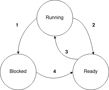
Fig. 8.1 The process life cycle showing the possible transitions between the states.

As shown in Fig. 8.1, there are three possible states for a process, and all the valid state transitions are represented by the arrows. A process in the Running state is one that is currently active on a CPU. A running process can move to either the ‘Ready’ or ‘Blocked’ state.

To move to the Blocked state (labeled 1), a process must take an action that cannot be completed immediately. Some examples of blocking operations are: issuing a read from disk or from a network socket that does not have data ready, issuing a write to a pipe that has no more space to buffer data, trying to acquire certain kinds of resources that are already owned by another process or thread, etc. In these situations, the process must wait for something external itself to happen before it can make progress (e.g., data arrives over the network, another process reads some data out of the pipe, the requested resource is released by another process, etc.), and is unable to make use of the CPU until that event occurs. We would be wasting the limited CPU resource if we left such a process on the CPU, and there is no point considering it among the set of runnable processes that we might want to choose next either. Thus, a Running process that takes an action that will block is immediately moved to the Blocked state, allowing another process to use the CPU while it waits.

The other transition out of the Running state is to the Ready state (labeled 2), which happens when the running process either voluntarily yields the remainder of its allotted time slice, or is forcibly removed from the CPU by the OS after exhausting its time slice (called preemption). Moving from Ready to Running (labeled 3) requires the OS to select the process as the next to execute and place it on a processor. The final transition is from Blocked to Ready (labeled 4), which happens when the blocking request is now complete or ready.

8.2. Performing a Context Switch

Earlier we described the data structures used to hold process information; now we need a way to change the active process on a CPU. When the OS decides to change the active process, all of the state associated with the outgoing process is cached in its process control block (PCB). Next the OS selects a new process to take the CPU and loads the incoming process state from its PCB and sets the CPU to run the incoming process from where it last left off.

Note that each context switch requires two processes to undergo one of the state transitions shown in Fig. 8.1: the currently executing process transitions out of the Running state, and the next process selected to execute transitions from Ready into Running.

Context switches are expensive for two reasons. First, there is CPU overhead to save the state (i.e., CPU registers) of the outgoing process, select the next process to run, and load the state of the incoming process. Second, even though we are saving all the state needed to resume a process, modern processors have several caches (e.g., data and instruction caches, the translation look aside buffer, etc.) that help a process run more quickly. As a process runs, these caches are filled with instructions or data that are related to the executing process. When a new process is placed on a CPU, the contents of these caches are no longer related to the running process, and either need to be cleared by the OS, or need to be replaced by the new process as it executes.

8.3. Considerations for Scheduling Policies

As we will see, a large number of scheduling policies have been developed over the years. Some of these are specialized for particular types of computing systems, while others aim to support more general-purpose systems. In this section, we will look at two broad categories of schedulers, and then discuss the different factors that the OS designer should take into consideration when developing a scheduling policy.

8.3.1. Batch versus Preemptive

Batch scheduling is a ‘run to completion’ model which means that once a job starts, it remains the active job on a CPU until it has completed. This mode of scheduling was used in early computers and is still used for some high-performance computing (HPC) systems. In our discussion of scheduling, we assume that batch jobs are finite, and will eventually complete. Preemptive scheduling is more familiar to the modern computer user because all consumer OS’s use this model. In a preemptive scheduling system we use the notion of the time slice; a process is only active on a CPU while it is not blocked and it has not exhausted its time slice. This allows us to build interactive systems that can respond to user input and can handle jobs with unbounded run time.

8.3.2. Factors in Process Selection

With all the parts in place to move processes on and off a CPU (i.e., the mechanism), we are only missing a method for choosing the next process to run on a CPU (i.e., the policy). Selecting the next process requires that the OS developer consider a number of possible criterion to optimize and to balance against each other. We must weigh things like responsiveness, turnaround time, throughput, predictability, fairness, and load on other parts of the system in making this decision, so let’s take a look at what each of these considerations are.

Responsiveness

Responsiveness is the amount of time required for the system to respond to an event or a request. If a user is interacting with the system, they will likely notice if the scheduler is not prioritizing responsiveness because they have to wait for key strokes or other input to have their effect.

Turnaround Time

Turnaround time is the amount of time between a job submission and its termination. Minimizing this time often helps with throughput.

Throughput

We define throughput as the number of processes completed per unit of time. To optimize for throughput, we want to ensure that the active process stays on the CPU as long as it isn’t blocked.

Predictability

We are not going to dive deeply into real-time computing, but there are classes of application which need to be certain of regular and predictable performance.

Note

Real-time scheduling is used in a wide class of applications from industrial controls to vehicle management to robotics. Predictability is a key requirement in each of these cases. Think of the program or programs responsible for managing an airplane in flight. The developers make decisions for the software with a guarantee that certain calculations can be made at least N times a second. If this requirement is not met, we start seeing bad and possibly dangerous behavior.

Fairness

Starvation in the context of scheduling is defined as a process never getting access to a CPU (for whatever reason). A functioning scheduler should not starve any process indefinitely. Achieving fairness may require more than simply not starving any process, however, we will use starvation-freedom as our fairness criteria.

These requirements are often in tension with each other and designing a scheduling algorithm is an act of balancing trade offs for the requirements of the OS.

8.4. Simple Examples of Scheduling Policies

Now that we have a collection of requirements, let’s look at a few simple possibilities and see which of our requirements they meet well and which ones they fail. Our first two examples are for batch system scheduling, which means that each job runs to completion before a new job is selected. All batch scheduling scheduling policies are optimized for throughput, since the CPU time spent on context switches is minimized and the time to complete each job is minimized.

The remaining examples are intended for preemptive scheduling.

8.4.1. First Come, First Served (FCFS)

Just like waiting in line at the local government office, each process gets into a queue and the processor executes the first process in that queue until it completes. Then we repeat the same. This method is really simple and it meets our fairness requirement as we can prove that no process will be stalled indefinitely. However, this policy has poor behavior when we mix short, CPU intensive jobs with longer or I/O bound jobs. If a terminal process has to wait in a queue behind a long compilation task, it could look to the user as if the terminal is not responding to key strokes. Also, turnaround time for a job in this scheduler is entirely based on the length of the jobs preceding it in the queue.

First come, first served meets our fairness requirement well, but it falls down on almost all the others.

8.4.2. Shortest Job First (SJF)

Instead of using arrival time for selecting the next process, we sort the queue of processes by the amount of time they will take to run, and we keep the queue sorted by inserting processes by run time. This algorithm improves turnaround time and throughput over first come, first served but we can construct scenarios where long-running jobs are stalled indefinitely by having short jobs continually arriving on the system. Knowing how long a job will take to run when it first arrives is an additional complication for shortest job first scheduling.

Shortest job first gives excellent throughput and can yield good turnaround time and responsiveness for systems with only short jobs. However, it totally fails on fairness and predictability.

8.4.3. Round Robin

Our first preemptive scheduling algorithm is just like first come, first served but we have added the time slice so processes are no longer run to completion. In this model, we still have a single queue of processes in the Ready state, and processes can be added to it upon creation or when leaving the Blocked state. When a process becomes active, it is given a fixed amount of time to run, and when this time slice expires the OS interrupts the process and puts it at the back of the queue.

Note

The preemptive scheduling models introduces a new parameter we need to set: the length of the time slice. We have to weigh the cost of changing processes against the interactivity requirements when deciding on the length of a time slice. Later on we will see systems that change the length based on usage patterns.

8.4.4. Priority

The core idea behind priority scheduling is that some processes may be more important than others and should be given access to the CPU first. To implement this policy, the OS maintains two or more priority queues which hold processes assigned to the corresponding priority. Runnable processes in a higher priority queue are run before runnable processes in lower priority queues. In general we assign higher priorities to I/O bound processes and lower priorities to CPU bound ones. Figure Fig. 8.2 shows a simple example of a system with 4 priority queues. In this snapshot, the next process to be given CPU time will be the first process in the priority 4 queue. Assuming no additions, the processes in queue 3 will not run until all of the ones in 4 have completed.

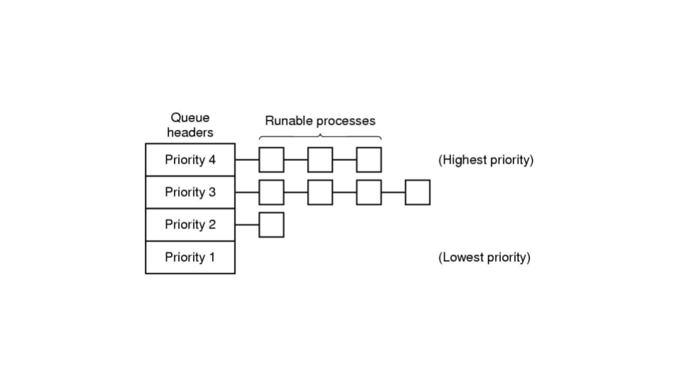
Fig. 8.2 A simple example of a system with 4 priority queues and runnable processes in several of the queues.

Note

It may seem counter-intuitive to assign high priority to I/O bound processes because they often do not make use of their full time slice. We do this because a process that is frequently blocking on I/O is more likely to be interactive and therefore have a user who will notice latency when the scheduler ignores the process for several periods.

8.4.5. Lottery

As the name suggests, in lottery scheduling the OS gives ‘tickets’ to each runnable process. When the scheduler needs to select a new process to run, it picks a ticket at random and the process holding that ticket runs. With a small modification, we can express priority in this method by assigning more tickets to high priority processes than low.

These examples are not exhaustive, there are other algorithms for selecting the next runnable process, however these examples are meant to illustrate that there are a number of ways to approach this problem and this is an active area of research today.